Table Of Contents
Intro Link to heading
I recently learned of Polars, which describes itself as a Lightning-fast DataFrame library for Rust and Python. It aims at having all the standard features you expect from a DataFrame library, while being extremely fast. They link a good benchmark for comparing different DataFrame libraries, done by h2o. Here is the benchmark from their site for a groupby and 5 GB dataset.
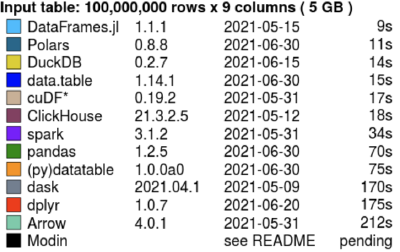
I use pandas frequently for typical DataFrame wrangling in Python. When I started using pandas I had recently converted to doing more Python than R so I was just looking for a library that was easy to use, not necessarily performant. I have been really happy with pandas over the years, it has a very expressive syntax and great documentation. The release of pandas 2.0 made significant performance improvements due to a swap of the backend to pyarrow. Learning about Polars made me wonder if I should have re-evaluated my usage of pandas before. Well there is no time like the present!
The benchmark that h2o did is pretty convincing, but I figured I would create a simple example that I could replicate across pandas, Polars, and pyarrow. For this simple comparison I grabbed a job postings dataset off of Kaggle. This simple benchmark is not thorough or particularly difficult. The dataset is only ~65mb in size. However, it covers basic manipulation including loading data from a csv, computing grouped aggregations, plotting, filtering, combining data, and sorting. I don’t know pyarrow or Polars well, so the functions I chose to achieve each of these steps might not be the best way.
Benchmarking code Link to heading
To start, here is reading in data and computing some simple statistics in pandas:
job_data = pd.read_csv('job_postings.csv')
grouped_wt = job_data.groupby(by='work_type')['med_salary']
salary_by_work_type = grouped_wt.agg(['min', 'median', 'max']).reset_index()
print(salary_by_work_type)
plot_med_salary(salary_by_work_type['median'], salary_by_work_type['work_type'], 'pandas_med_plot.png')
This is straightforward: read data, group by the work_type, compute stats for the med_salary, and then plot it. The plotting function is the same across the use cases; the only thing that differs is accessing the data.
Doing the same thing in Polars looks mostly similar, though a bit more verbose:
job_data = pl.read_csv('job_postings.csv')
grouped_wt = job_data.group_by("work_type").agg(
    pl.min("med_salary").alias('min'),
    pl.median("med_salary").alias('median'),
    pl.max("med_salary").alias('max')
)
print(grouped_wt)
plot_med_salary(grouped_wt['median'], grouped_wt['work_type'], 'polars_med_plot.png')
Because I am computing 3 statistics for the same column, the alias function has to be used to give them different names. Otherwise, they would all be called med_salary in the result.
Here is pyarrow:
job_data = csv.read_csv('job_postings.csv', parse_options=csv.ParseOptions(newlines_in_values=True))
groupted_wt = pa.TableGroupBy(job_data, "work_type")
salary_by_work_type = groupted_wt.aggregate([("med_salary", "min"), ("med_salary", "approximate_median"), ("med_salary", "max")])
print(salary_by_work_type)
plot_med_salary(salary_by_work_type['med_salary_approximate_median'], salary_by_work_type['work_type'], 'pyarrow_med_plot.png')
The pyarrow version is pretty comparable to pandas, just a bit more verbose in aggregate syntax. Note pandas and Polars could read the data fine as is, but pyarrow had to be told to allow newlines in csv values to read it in.
From here, I did combining data: I kept it simple with having the same columns, just stacking. For pandas this is done with a for loop and a list:
frames = []
for i in range(10):
    frames.append(sales_mgr_jobs)
    frames.append(software_jobs)

comb_jobs = pd.concat(frames)
Polars has a nice way to do this inline, avoiding having to keep a separate list:
combined = sales_mgr_jobs
for _ in range(10):
    combined.vstack(sales_mgr_jobs, in_place=True)
    combined.vstack(software_jobs, in_place=True)
Pyarrow again looks very similar to pandas:
frames = []
for i in range(10):
    frames.append(sales_mgr_jobs)
    frames.append(software_jobs)

comb_jobs = pa.concat_tables(frames)
Finally for sorting, I just sorted the original data by the med_salary. In retrospect maybe I should have done this with the combined data for a bit harder test. Here are all the methods together, to keep it shorter:
job_data = job_data.sort_values('med_salary') #pandas
job_data = job_data.sort("med_salary") #Polars
job_data = job_data.sort("med_salary") #pyarrow
Overall the syntax between the libraries is very comparable. The docs for each library are all pretty good. Polars was a little light on examples, but the apidocs were more than enough to figure out what I needed. Besides the aggregate syntax shown, I found that pandas was the most concise for computing quantiles across all the numeric fields of the data. With 1 line, this can be done using a list of quantiles. Polars required three, one for each quantile I wanted to compute. Whereas, with pyarrow, I couldn’t figure out a nice way to do this, so I used list comprehension:
numeric_fields = [f.name for f in job_data.schema if not f.type.equals(pa.string())]
jd_quant = [pc.quantile(job_data[f], [.1, .5, 0.9], interpolation="nearest") for f in numeric_fields]
Results Link to heading
As I said the example was pretty simple. How did each library do? I profiled the time for each library using cProfile and the memory using the memory-profiler library. For time, I ran each example 1 time and 100 times. This was so I could get a better feel for the stability of the performance and hopefully not have any unlucky cpu scheduling issues messing with my data. The results are below:
| library | 1 run time (s) | 100 run time (s) |
|---|---|---|
| pandas | 0.749 | 65.9 |
| Polars | 0.283 | 17.3 |
| pyarrow | 0.207 | 11.8 |
Both Polars and pyarrow blew pandas out of the water. With 1 run, they are all less than 1s, so a user likely wouldn’t notice. However, with 100 runs, there is a noticable difference waiting for my script to run. I did visualize each of the profiles using snakeviz. For pandas, since it was the slowest, here is a snakeviz with the 100x run.
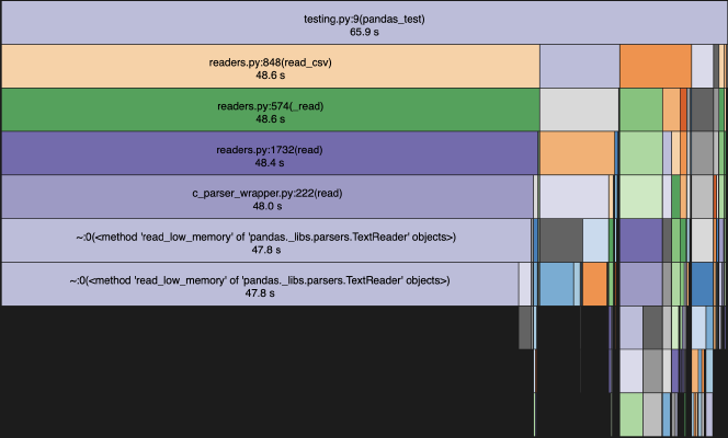
As you can see the vast majority of the time is spent reading in the csv.
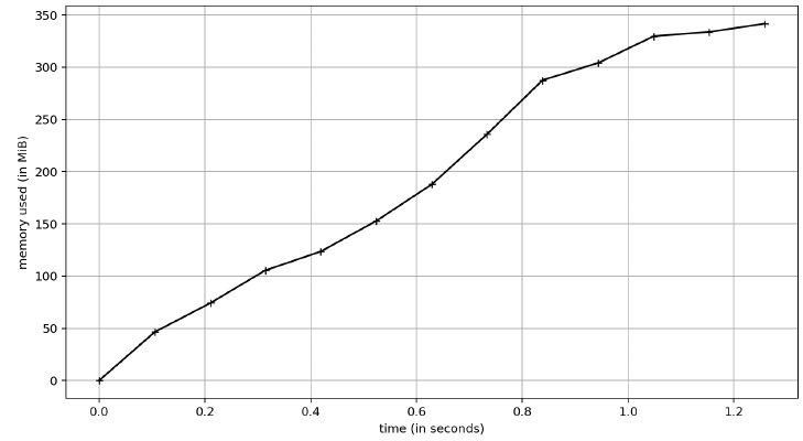
For the memory profiles here is pandas:
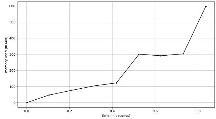
Polars:
and pyarrow:
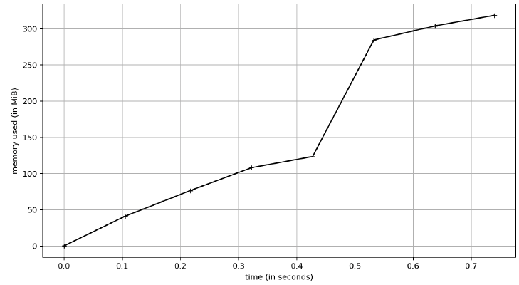
For this profile, I just did 1 run and captured the memory. Because I wanted to ensure I did it right, however, I did rerun the Polars test a few times. As you can see, pyarrow and pandas use the same amount of memory (~350MB) whereas Polars is using 600MB. I did look at the line profile for this and Polars doubles its memory usage with the sort call. So if you don’t have to sort, then they are all comparable memory-wise. Python is a garbage collected language and my simple test here didn’t last long enough to see that happen, so over the lifetime of an application the differences might be non-existent.
Summary Link to heading
Based off my very simple example, I am going to have to really consider swapping my usage of pandas to Polars or pyarrow. For simple things, I will likely still use pandas, but anything with lots of data or more complex computation it seems worth it to swap over. I learned of Polars due to an announcement that they are starting a company, so it seems like long-time support of both pyarrow and Polars is great. The source for my simple tests can be found here.